How to?
In this section, we are providing a summary of what actions or modification need to be done in order to answer your simulation problem.
Visualizing Simulation
If CoordinatesFreq is enabled in configuration file, GOMC will output the molecule coordinates every
specified stpes. The PDB and PSF output (merging of atom entries) has already been mentioned/explained in
previous sections. To recap: The PDB file’s ATOM entries’ occupancy is used to represent the box the molecule
is in for the current frame. All molecules are listed in order in which they were read (i.e. if box 0 has
\(1, 2, ..., N1\) molecules and box 1 has \(1, 2, ..., N2\) molecules, then all of the molecules in
box 0 are listed first and all the molecules in box 1, i.e. \(1, 2 ,... ,N1\), \(N1 + 1, ..., N1 + N2\)).
PDB frames are written as standard PDBs to consecutive file frames.
To visualize, open the output PDB and PSF files by GOMC using VMD, type this command in the terminal:
For all simulation except Gibbs ensemble that has one simulation box:
$ vmd ISB_T_270_k_merged.psf ISB_T_270_k_BOX_0.pdb
For Gibbs ensemble, visualizing the first box:
$ vmd ISB_T_270_k_merged.psf ISB_T_270_k_BOX_0.pdb
For Gibbs ensemble, visualizing the second box:
$ vmd ISB_T_270_k_merged.psf ISB_T_270_k_BOX_1.pdb
Note
Restart coordinate file (OutputName_BOX_0_restart.pdb) cannot be visualize using merged psf file, because atom number does not match. However, you can still open it in vmd using following command and vmd will automatically find the bonds of the molecule based on the coordinates.
$ vmd ISB_T_270_k_BOX_0_restart.pdb
Build molecule and topology file
There are many open-source software that can build a molecule for you, such as Avagadro , molefacture in VMD and more. Here we use molefacture features to not only build a molecule, but also creating the topology file.
Regular molecule
First, make sure that VMD is installed on your computer. Then, to learn how to build a single PDB file and topology file for united atom butane molecule, please refer to this document .
We encourage to try to go through our workshop materials:
To try two days workshop, execute the following command in your terminal to clone the workshop:
$ git  clone    https://github.com/GOMC-WSU/Workshop.git --branch master --single-branch
$ cd   Workshop
or simply download it from GitHub .
To try two hours workshop, execute the following command in your terminal to clone the workshop:
$ git  clone    https://github.com/GOMC-WSU/Workshop.git --branch AIChE --single-branch
$ cd   Workshop
or simply download it from GitHub .
Molecule with dummy atoms
To simulate a molecule that includes one or more atoms with electrostatic interaction only and no LJ interaction (i.e. dummy atom near of the oxygen along the bisector of the HOH angle in TIP4P water model), we must perform the following steps to define the dummy atom/atoms:
Create a PDB file for single water molecule atoms (H1, O, H2) and a dummy atom (M, in this example), where dummy atom located at 0.150 Å of oxygen and along the bisector of the H1-O-H2 angle.
CRYST1    0.000    0.000    0.000  90.00  90.00  90.00 P 1           1
ATOM      1  O   TIP4    1      -0.189   1.073   0.000  0.00  0.00           O
ATOM      2  H1  TIP4    1       0.768   1.114   0.000  0.00  0.00           H
ATOM      3  H2  TIP4    1      -0.469   1.988   0.000  0.00  0.00           H
ATOM      4  M   TIP4    1      -0.102   1.195   0.000  0.00  0.00           D
END
Pack your desire number of TIP4 water molecule in a box using packmol, as explained before.
Include the dummy atom (M) and its charge in your topology file. Define a bond between oxygen and dummy atom. Use vmd and build script to generate your PSF files.
* Custom top file -- TIP4P water

MASS   1  OH    15.9994  O !
MASS   2  HO     1.0080  H !
MASS   3  MO     0.0000  D ! Dummy atom for TIP4P model

DEFA FIRS none LAST none
AUTOGENERATE ANGLES DIHEDRALS

RESI TIP4           0.0000 ! TIP4P water
GROUP
ATOM O      OH      0.0000 !        O
ATOM H1     HO      0.5564 !     /  |  \
ATOM H2     HO      0.5564 !    /   M   \
ATOM M      MO     -1.1128 !  H1        H2
BOND   O  H1   O  H2   O  M
PATCHING FIRS NONE LAST NONE

END
Define all bonded parameters (bond, angles, and dihedral) and nonbonded parameters in your parameter file.
*parameteres for TIP4P

BONDS
!
!V(bond) = Kb(b - b0)**2
!
!atom type          Kb          b0
OH   HO    99999999999       0.9572 ! TIP4P O-H bond length
OH   MO    99999999999       0.1500 ! TIP4P M-O bond length


ANGLES
!
!V(angle) = Ktheta(Theta - Theta0)**2
!
!atom types         Ktheta       Theta0
HO   OH   HO    9999999999999    104.52  ! H-O-H Fix Angle
HO   OH   MO    9999999999999     52.26  ! H-O-M Fix Angle


DIHEDRALS
!
!V(dihedral) = Kchi(1 + cos(n(chi) - delta))
!
!atom types             Kchi    n   delta


NONBONDED
!
!V(Lennard-Jones) = Eps,i,j[(Rmin,i,j/ri,j)**12 - 2(Rmin,i,j/ri,j)**6]
!
!atom  ignored      epsilon      Rmin/2   ignored   eps,1-4    Rmin/2,1-4
HO      0.000000     0.00000    0.000000    0.0     0.0         0.0
MO      0.000000     0.00000    0.000000    0.0     0.0         0.0
OH      0.000000    -0.18521    1.772873    0.0     0.0         0.0
Simulate rigid molecule
Currently, GOMC can simulate rigid molecules for any molecular topology in NVT and NPT ensemble, if none of the Monte Carlo moves that lead to change in
molecular configuration (e.g. Regrowth, Crankshaft, IntraSwap, and etc.) was used.
In general, GOMC can simulate rigid molecules in all ensembles for the following molecular topology:
Linear and branched molecules with no dihedrals. For instance, carbon dioxide, dimethyl ether, and all water models (SPC, SPC/E, TIP3P, TIP4P, etc).
Cyclic molecules, where at least two atoms in all defined angles, belong to the body of the ring. For instance, benzene, toluene, Xylene, and more.
Important
For linear and branched molecule, the molecule’s bonds and angles will be adjusted according to the equilibrium values, defined in parameter file.
For cyclic molecules, the molecule’s bonds and angles would not change! It is very important to create the initial molecule with correct bonds and angles.
Setup rigid molecule
To simulate the rigid molecules in GOMC, we need to perform the following steps:
Define all bonds in topology file and use AUTOGENERATE ANGLES DIHEDRALS in topology file to specify all angles and dihedral in PSF files.
Define all bond parameters in the parameter file. If you wish to not to include the bond energy in your simulation, set the the \(K_b\) to a large value i.e. “999999999999”.
Define all angle parameters in the parameter file. If you wish to not to include the bend energy in your simulation, set the the \(K_{\theta}\) to a large value i.e. “999999999999”.
Define all dihedral parameters in parameter file. If you wish to not to include the dihedral energy in your simulation, set the all the \(C_n\) to zero. For cyclic molecules only
Restart the simulation
Restart the simulation with Restart
If you intend to start a new simulation from previous simulation state, you can use this option. Restarting the simulation with Restart would not result in
an identical outcome, as if previous simulation was continued.
Make sure that in the previous simulation config file, the flag RestartFreq was activated and the restart PDB file/files (OutputName_BOX_0_restart.pdb)
and restart PSF file file/files (OutputName_BOX_0_restart.psf) were printed.
In order to restart the simulation from previous simulation we need to perform the following steps to modify the config file:
Set the
Restartto True.Use the restart PDB file/files to set the
Coordinatesfor each box.Use the restart PSF file/files to set the
Structurefor each box.Use the restart xsc file/files to set the
extendedSystemfor each box.Use the restart coor file/files to set the
binCoordinatesfor each box.It is a good practice to comment out the
CellBasisVectorby adding ‘#’ at the beginning of each cell basis vector. However, GOMC will override the cell basis information with the cell basis data from restart PDB file/files.Use the different
OutputNameto avoid overwriting the output files.
Here is the example of starting the NPT simulation of dimethyl ether, from equilibrated NVT simulation:
########################################################
# Parameters need to be modified
########################################################
Restart         true

Coordinates     0   dimethylether_NVT_BOX_0_restart.pdb

Structure       0   dimethylether_NVT_BOX_0_restart.psf

extendedSystem  0   dimethylether_NVT_BOX_0_restart.xsc

binCoordinates  0   dimethylether_NVT_BOX_0_restart.coor

#CellBasisVector1   0       45.00   0.00    0.00
#CellBasisVector2   0       0.00    55.00   0.00
#CellBasisVector3   0       0.00    0.00    45.00

OutputName          dimethylether_NPT
Here is the example of starting the NPT-GEMC simulation of dimethyl ether, from equilibrated NVT simulation:
########################################################
# Parameters need to be modified
########################################################
Restart         true

Coordinates     0   dimethylether_NVT_BOX_0_restart.pdb
Coordinates     1   dimethylether_NVT_BOX_1_restart.pdb

Structure       0   dimethylether_NVT_BOX_0_restart.psf
Structure       1   dimethylether_NVT_BOX_1_restart.psf

extendedSystem  0   dimethylether_NVT_BOX_0_restart.xsc
extendedSystem  1   dimethylether_NVT_BOX_1_restart.xsc

binCoordinates  0   dimethylether_NVT_BOX_0_restart.coor
binCoordinates  1   dimethylether_NVT_BOX_1_restart.coor

#CellBasisVector1   0       45.00   0.00    0.00
#CellBasisVector2   0       0.00    55.00   0.00
#CellBasisVector3   0       0.00    0.00    45.00

#CellBasisVector1   1       45.00   0.00    0.00
#CellBasisVector2   1       0.00    55.00   0.00
#CellBasisVector3   1       0.00    0.00    45.00

OutputName          dimethylether_NPT_GEMC
Restart the simulation with Checkpoint
If you intend to continue your simulation from previous simulation, you can use this option. Restarting the simulation with Checkpoint would result in an
identical outcome, as if previous simulation was continued.
Make sure that in the previous simulation config file, the flag RestartFreq was activated and the restart PDB file/files (OutputName_BOX_N_restart.pdb)
, restart PSF file/files (OutputName_BOX_N_restart.psf), binary coodinate file/files (OutputName_BOX_N_restart.coor), XSC file/files (OutputName_BOX_N_restart.xsc) was printed.
Make sure that in the previous simulation config file, the flag CheckpointFreq was activated and the checkpoint file (OutputName_restart.chk) was printed.
Make sure that in the CheckpointFreq equals the RestartFreq.
In order to restart the simulation from previous simulation we need to perform the following steps to modify the config file:
Set the
Restartto True.Set the
Checkpointto True and provide the Checkpoint file.Use the restart PDB file/files to set the
Coordinatesfor each box.Use the restart PSF file/files to set the
Structurefor each box.Use the restart xsc file/files to set the
extendedSystemfor each box.Use the restart coor file/files to set the
binCoordinatesfor each box.It is a good practice to comment out the
CellBasisVectorby adding ‘#’ at the beginning of each cell basis vector. However, GOMC will override the cell basis information with the cell basis data from XSC file/files.Use the different
OutputNameto avoid overwriting the output files.
Here is the example of restarting the NPT simulation of dimethyl ether, from equilibrated NVT simulation:
########################################################
# Parameters need to be modified
########################################################
Restart         true

Checkpoint   true   dimethylether_NVT_restart.chk

Coordinates     0   dimethylether_NVT_BOX_0_restart.pdb

Structure       0   dimethylether_NVT_BOX_0_restart.psf

extendedSystem   0   dimethylether_NVT_BOX_0_restart.xsc

binCoordinates   0   dimethylether_NVT_BOX_0_restart.coor

#CellBasisVector1   0       45.00   0.00    0.00
#CellBasisVector2   0       0.00    55.00   0.00
#CellBasisVector3   0       0.00    0.00    45.00

OutputName          dimethylether_NPT
Here is the example of restarting the NPT-GEMC simulation of dimethyl ether, from equilibrated NVT simulation:
########################################################
# Parameters need to be modified
########################################################
Restart         true

Checkpoint   true   dimethylether_NVT_restart.chk

Coordinates     0   dimethylether_NVT_BOX_0_restart.pdb
Coordinates     1   dimethylether_NVT_BOX_1_restart.pdb

Structure     0   dimethylether_NVT_BOX_0_restart.psf
Structure     1   dimethylether_NVT_BOX_1_restart.psf

extendedSystem   0   dimethylether_NVT_BOX_0_restart.xsc
extendedSystem   1   dimethylether_NVT_BOX_1_restart.xsc

binCoordinates   0   dimethylether_NVT_BOX_0_restart.coor
binCoordinates   1   dimethylether_NVT_BOX_1_restart.coor

#CellBasisVector1   0       45.00   0.00    0.00
#CellBasisVector2   0       0.00    55.00   0.00
#CellBasisVector3   0       0.00    0.00    45.00

#CellBasisVector1   1       45.00   0.00    0.00
#CellBasisVector2   1       0.00    55.00   0.00
#CellBasisVector3   1       0.00    0.00    45.00

OutputName          dimethylether_NPT_GEMC
Note
As of right now, restarting is not supported for Multi-Sim.
Recalculate the energy
GOMC is capable of recalculate the energy of previous simulation snapshot, with same or different force field. Simulation snapshot is the printed molecule’s
coordinates at specific steps, which controls by CoordinatesFreq. First, we need to make sure that in the previous simulation config file, the flag CoordinatesFreq
was activated and the coordinates PDB file/files (OutputName_BOX_0.pdb) and merged PSF file (OutputName_merged.psf) were printed.
In order to recalculate the energy from previous simulation we need to perform the following steps to modify the config file:
Set the
Restartto True.Use the dumped coordinates PDB file to set the
Coordinatesfor each box.Use the dumped merged PSF file to set the
Structurefor both boxes.Set the
RunStepsto zero to activare the energy recalculation.Use the different
OutputNameto avoid overwriting the merged PSF files.
Note
GOMC only recalculated the energy terms and does not recalulate the thermodynamic properties. Hence, no output file, except merged PSF file, will be generated.
Here is the example of recalculating energy from previous NVT simulation snapshot:
########################################################
# Parameters need to be modified
########################################################
Restart         true

Coordinates     0   dimethylether_NVT_BOX_0.pdb

Structure       0   dimethylether_NVT_merged.psf

RunSteps        0

OutputName          Recalculate
Simulate adsorption
GOMC is capable of simulating gas adsorption in rigid framework using GCMC and NPT-GEMC simulation. In this section, we discuss how to generate PDB and PSF file, how to modify the configuration file to simulate adsorption.
Build PDB and PSF file
Generating PDB and PSF file for reservoir is similar to generating PDB and PSF file for isobutane, explained before. Here, we are focusing on how to generate PDB and PSF file for adsorbent. As mensioned before, GOMC can only read PDB and PSF file as input file. If you are using “*.cif” file for your adsorbent, you need to perform few steps to extend the unit cell and export it as PDB file. There are two ways that you can prepare your adsorption simulation:
Using High Throughput Screening (HTS)
GOMC development group created a python code combined with Tcl scripting to automatically generate GOMC input files for adsorption simulation. In this code, we use CoRE-MOF repository created by Snurr et al. to prepare the simulation input file.
To try this code, execute the following command in your terminal to clone the HTS repository:
$ git  clone    https://github.com/GOMC-WSU/Workshop.git --branch HTS --single-branch
$ cd   Workshop
or simply download it from GitHub .
Make sure that you installed all GOMC software requirement. Follow the “Readme.md” for more information.
Manual Preparation
To illustrate the steps that need to be taken to prepare the PDB and PSF file, we will use an example provided in one of our workshop. Make sure that you installed all GOMC software requirement.
To clone the workshop, execute the following command in your terminal to clone the workshop:
$ git clone https://github.com/GOMC-WSU/Workshop.git --branch master --single-branch
or simply download it from GitHub .
To show how to extend the unit cell of IRMOF-1 and build the PDB and PSF files, change your directory to:
$ cd Workshop/adsorption/GCMC/argon_IRMOF_1/build/base/.In this directory, there is a “README.txt” file, which provides detailed information of steps need to be taken. Here we just provide a summary of these steps:
Extend the unit cell of “EDUSIF_clean_min.cif” file using VESTA. To learn how to extend the unit cell, removing bonds, and export it as PDB file, please refere to this documente to generate “EDUSIF_clean_min.pdb” file.
Note
Generated PDB file does not provide all necessary information. Further modification must be made.
The easy way to generate PSF file is to treat each atom as a separate molecule kind to avoid defining bonds, angles, and dihedrals. To modify the “EDUSIF_clean_min.pdb” file (set the residue ID, resname, …), execute the following command to generate the “EDUSIF_clean_min_modified.pdb” file.
vmd -dispdev text < convert_VESTA_PDB.tcl
Treating each atom as separate molecule kind will make it easy to generate topology file. Here is an example of topology file where each atom is treated as a separate residue kind:
* Topology file for IRMOF-1 (Zn4O(BDC)3)
!
MASS   1  O     15.999      O  !
MASS   2  C     12.011      C  !
MASS   3  H      1.008      H  !
MASS   4  ZN    65.380      ZN !

DEFA FIRS none LAST none
AUTOGENERATE ANGLES DIHEDRALS

RESI    C         0.000
GROUP
ATOM    C   C     0.000
PATCHING FIRS NONE LAST NONE

RESI    H         0.000
GROUP
ATOM    H   H     0.000
PATCHING FIRS NONE LAST NONE

RESI    O          0.000
GROUP
ATOM    O   O      0.000
PATCHING FIRS NONE LAST NONE

RESI    Zn         0.000
GROUP
ATOM    Zn  ZN     0.000
PATCHING FIRS NONE LAST NONE

END
To generate the PSF file, each molecule kind must be separated and stored in separate pdb file. Then we use VMD to generate the PSF file. All these process are scripted in “build_EDUSIF_auto.tcl” and we just need to execute the following command to generate the “IRMOF_1_BOX_0.pdb” and “IRMOF_1_BOX_0.psf” files.
vmd -dispdev text < build_EDUSIF_auto.tcl
Last steps to fix the adsorbent atoms in their position. As mensioned in PDB section, setting the
Beta = 1.00value of a molecule in PDB file, will fix that molecule position. This can be done by a text editor but here we use another Tcl scrip to do that. Execute the following command in your terminal to set theBetavalue of all atoms in “IRMOF_1_BOX_0.pdb” to 1.00.
vmd -dispdev text < setBeta.tcl
Adsorption in GCMC
To simulate adsorption using GCMC ensemble, we need to perform the following steps to modify the config file:
Use the generated PDB files for adsorbent and adsorbate to set the
Coordinates.Use the generated PSF files for adsorbent and adsorbate to set the
Structure.Calculate the cell basis vectors for each box and set the
CellBasisVector1,2,3for each box.
Note
To calculate the cell basis vector with cell length \(\boldsymbol{a} , \boldsymbol{b}, \boldsymbol{c}\) and cell angle \(\alpha, \beta. \gamma\) we use the following equations:
\(a_x = \boldsymbol{a}\)
\(a_y = 0.0\)
\(a_z = 0.0\)
\(b_x = \boldsymbol{b} \times cos(\gamma)\)
\(b_y = \boldsymbol{b} \times sin(\gamma)\)
\(c_x = \boldsymbol{c} \times cos(\beta)\)
\(c_y = \boldsymbol{c} \times \frac{ cos(\alpha) - cos(\beta) \times cos(\gamma) } { sin(\gamma) }\)
\(c_z = \boldsymbol{c} \times \sqrt {{sin(\beta)}^2 - { \bigg(\frac{ cos(\alpha) - cos(\beta) \times cos(\gamma) } { sin(\gamma) }} \bigg)^2}\)
CellBasisVector1 = \((a_x , a_y, a_z)\)
CellBasisVector2 = \((b_x , b_y, b_z)\)
CellBasisVector3 = \((c_x , c_y, c_z)\)
Set the
Fugacityfor adsorbate and includeFugacityfor adsorbent with arbitrary value (e.g. 0.00).
Here is the example of argon (AR) adsorption at 5 bar in IRMOF-1 using GCMC ensemble:
########################################################
# Parameters need to be modified
########################################################
Coordinates     0   ../build/base/IRMOF_1_BOX_0.pdb
Coordinates     1   ../build/reservoir/START_BOX_1.pdb

Structure       0   ../build/base/IRMOF_1_BOX_0.psf
Structure       1   ../build/reservoir/START_BOX_1.psf

CellBasisVector1    0   36.8140   0.00     0.00
CellBasisVector2    0   18.2583  31.9880   0.00
CellBasisVector3    0   18.2712  10.5596  30.1748

CellBasisVector1    1   40.00     0.00    0.00
CellBasisVector2    1    0.00    40.00    0.00
CellBasisVector3    1    0.00    00.00   40.00

Fugacity    AR      5.0
Fugacity    C       0.0
Fugacity    H       0.0
Fugacity    O       0.0
Fugacity    ZN      0.0
Adsorption in NPT-GEMC
To simulate adsorption using NPT-GEMC ensemble, simulaiton box 0 is used for adsorbent with fixed volume and simulaiton box 1 is used for adsorbate, where volume of this box is fluctuating at imposed pressure. To simulation adsorption in NPT-GEMC ensemble we need to perform the following steps to modify the config file:
Use the generated PDB file for adsorbent to set the
Coordinatesfor box 0.Use the generated PDB file for adsorbate to set the
Coordinatesfor box 1.Use the generated PSF file for adsorbent to set the
Structurefor box 0.Use the generated PSF file for adsorbate to set the
Structurefor box 1.Calculate the cell basis vectors for each box and set the
CellBasisVector1,2,3for each box.Set the
GEMCsimulaiton type to “NPT”.Set the imposed
Pressure(bar) for fluid phase.Keep the volume of box 0 constant by activating the
FixVolBox0.
Here is the example of argon (AR) adsorption at 5 bar in IRMOF-1 using NPT-GEMC ensemble:
########################################################
# Parameters need to be modified
########################################################
Coordinates     0   ../build/base/IRMOF_1_BOX_0.pdb
Coordinates     1   ../build/reservoir/START_BOX_1.pdb

Structure       0   ../build/base/IRMOF_1_BOX_0.psf
Structure       1   ../build/reservoir/START_BOX_1.psf

CellBasisVector1    0   36.8140   0.00     0.00
CellBasisVector2    0   18.2583  31.9880   0.00
CellBasisVector3    0   18.2712  10.5596  30.1748

CellBasisVector1    1   40.00     0.00    0.00
CellBasisVector2    1    0.00    40.00    0.00
CellBasisVector3    1    0.00    00.00   40.00

GEMC        NPT

Pressure    5.0

FixVolBox0  true
Calculate Solvation Free Energy
GOMC is capable of calcutating absolute solvation free energy in NVT or NPT ensemble. Here we are focusing how to setup the GOMC simulation files to calculate absolute solvation free energy.
GOMC outputs the required informations (\(\frac{dE_{\lambda}}{d\lambda}\), \(\Delta E_{\lambda}\)) to calculate solvation free energy with various estimators, such as TI, BAR, MBAR, and more.
Setup Simulation Files
Using FreeEnergy BASH Script
GOMC development group created a BASH script combined with Tcl scripting to automatically generate GOMC input files for free energy simulations in NVT (master branch) or NPT (NPT branch) ensemble.
To try this script, execute the following command in your terminal to clone the FreeEnergy repository:
$ git  clone    https://github.com/msoroush/FreeEnergy.git
$ cd   FreeEnergy
or simply download it from GitHub .
Make sure that you installed all GOMC software requirement. Follow the README for more information.
Manual Preparation
To simulate solvation free energy, we need to perform the following steps:
Generate the PDB and PSF files for a system containes 1 solulte + N solvent molecules.
Note
Number of solvent molecules (N) must be determined by user, based on the system size.
Equilibrate your system in NVT ensemble at specified
Temperature.Equilibrate your system in NPT ensemble at specified
TemperatureandPressure, using PDB and PSFrestartfiles, generated from previous equilibration simulation.Determine the number of intermediate states that lead to adequate overlaps between neighboring states.
For each intermediate state (\(\lambda_i\)), create an unique directory and perform the following steps:
Use the
restartPDB file, generated from NPT equilibration simulation, to set theCoordinates.Use the
mergedPSF files, generated from NPT equilibration simulation, to set theStructure.Define the free energy parameters in
configfile:Set the frequency of free energy calculation
Set the solute molecule kind name (resname) and number (resid)
Set the soft-core parameters
Define the lambda vecotrs for
VDWandCoulombinteractionSet the index (\(i\)) of the lambda vetor (\(\lambda\)), at which solute-solvent interaction will be coupled with \(\lambda_i\), using
InitialStatekeyword.
Here is the example of free energy parameters for CO2 (resid 1) solvation, with 9 intermediate states, where the solute-solvent interaction will be coupled with \(\lambda_{\texttt{VDW}}(6)= 1.0\) , \(\lambda_{\texttt{Elect}}(6)= 0.50\).
#################################
# FREE ENERGY PARAMETERS
#################################
FreeEnergyCalc true   1000
MoleculeType   CO2   1
InitialState   6
ScalePower     2
ScaleAlpha     0.5
MinSigma       3.0
ScaleCoulomb   false
#states        0    1    2    3    4    5    6    7    8
LambdaVDW      0.00 0.25 0.50 0.75 1.00 1.00 1.00 1.00 1.00
LambdaCoulomb  0.00 0.00 0.00 0.00 0.00 0.25 0.50 0.75 1.00
Equilibrate your system in NVT or NPT ensemble.
Perform the production simulation in NVT or NPT ensemble.
Process GOMC Free Energy Outputs
I free energy perturbation method, the free energy difference between two states A (\(\lambda = 0.0\)) and B (\(\lambda = 1.0\)), with N - 2 intermediate states is given by:
where \(\Delta E_{i, i+1} = E_{i+1} - E_{i}\) is the energy difference of the system between states i and i+1, and \(\big< \big>_i\) is the ensemble average for simulation performed in intermediate state i.
In thermodynamic integration, the free energy change is calculated from
where \(\frac{dU_{\lambda}}{d\lambda}\) is the derivative of energy with respect to \(\lambda\), and \(\big< \big>_{\lambda}\) is the ensemble average for a simulation run at intermediate state \(\lambda\).
GOMC outputs the raw informations, such as the lambda intermediate states, the derivative of energy with respective to current lambda (\(\frac{dE_{\lambda}}{d\lambda}\)), the energy different between current lambda state and all other neighboring lambda states (\(\Delta E_{\lambda}\)), which is essential to calculate solvation free energy with various estimators, such as TI, BAR, MBAR, and more.
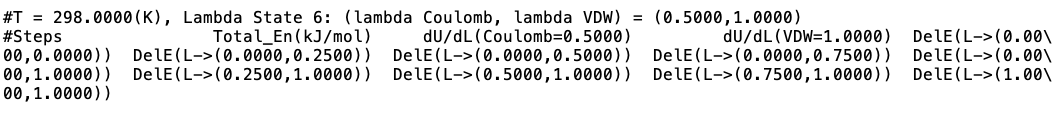
Snapshot of GOMC free energy output file (Free_Energy_BOX_0_ OutputName.dat).
There are variety of tools developed to caclulate free energy difference, including alchemlyb and alchemical-analysis .
Alchemlyb
In alchemlyb , a variety of methods can be used to estimate the free energy, including thermodynamic integration (TI), Bennett acceptance ratio (BAR), and multistate Bennett acceptance ratio (MBAR). alchemlyb is also capable of loading GOMC free energy output files (Free_Energy_BOX_0_
OutputName.dat).To learn more about alchemlybe, please refere to alchemlyb documentation or alchemlyb GitHub page.
Note
Currently, alchemlyb does not support the free energy plots, overlap analysis, and free energy convergance analysis.
To use this tool, you must install python 3 and then execute the following command in your terminal to install alchemlyb:
$ pip install alchemlyb
Alchemical Analysis
The alchemical-analysis tools is developed by Mobley group at MIT, to Analyze alchemical free energy calculations conducted in GROMACS, AMBER or SIRE. Alchemical Analysis is still available but deprecated and in the process of migrating all functionality to alchemlyb tool.
Alchemical Analysis tool handles analysis via a slate of free energy methods, including BAR, MBAR, TI, and the Zwanzig relationship (exponential averaging) among others, and provides a good deal of analysis of computed free energies and convergence in order to help you assess the quality of your results.
Since alchemical-analysis is no longer supported by its developers, the GOMC parser for this tool was implemented and stored in a separate repository.
Note
We encourage user to use alchemlyb GitHub tools for plotting, once all the plotting features and free energy analysis was migrated.
To use this tool, you must install python 2 and then execute the following command in your terminal to clone the alchemical-analysis repository:
$ git  clone    https://github.com/msoroush/alchemical-analysis.git
$ cd   alchemical-analysis
$ sudo python setup.py install
Run a Multi-Sim
GOMC can automatically generate independent simulations with varying temperatures from one input file. This allows the user to sample a wider seach space. To do so GOMC must be compiled in MPI mode, and a couple of parameters must be added to the conf file.
To compile in MPI mode, navigate to the GOMC/ directory and issue the following commands:
$ chmod u+x metamakeMPI.sh
$ ./metamakeMPI.sh
Then once the compilation is complete, set up the conf file as you would for a standard GOMC simulation.
Finally, enter more than one value for Temperature separated by a tab or space.
#################################
# SIMULATION CONDITION
#################################
Temperature   270.00    280.00    290.00    300.00
A folder will be created for the output of each simulation, and the name will be generated from the temperatures you choose.
A parent folder containing all the child folders will be created so as to not overpopulate the initial directory.
You may elect to choose the name of the folder in which all the sub-folders for each replica are contained.
Enter this name as a string following the MultiSimFolderName parameter. If you don’t provide this parameter, the default “MultiSimFolderName” will be used.
MultiSimFolderName outputFolderName
Note
To perform a multisim, GOMC must be compiled in MPI mode. Also, if GOMC is compiled in MPI mode, a multisim must be performed. To perform a standard simulation, use standard GOMC.
The rest of the conf file should be similar to how you would set up a standard GOMC simulation.
To initiate the multi-sim, first decide how many MPI processes and openMP threads you want to use and call GOMC with the following format.
$ mpiexec -n #ofsimulations GOMC_xxx_yyyy +p<#ofthreads>(optional) conffile
The number of MPI processes must equal the number of simulations you wish to run. Each will by default be assigned one openMP thread; however, if you have leftover processors, you may assign them as openMP threads. There must be an equal amount of openMP threads assigned to each process.
A formula to determine how many threads to use is as follows:
Floor[ ] - Rounds down a real number to the nearest integer.
For example, if I have 7 processors and I wanted to run 2 simulations in my multi-sim.
$ mpiexec -n 2 ./GOMC_CPU_GEMC +p2 in.conf
Simulate a protein as a fixed body
GOMC supports simulating a protein as a fixed body for solvation in complex solvents. There is experimental support for conformation sampling using the crankshaft and regrowth moves.
To simulate a rigid protein in GOMC, we need to perform the following steps:
Generate the PDB and PSF files for the system with protein centered in the box.
Ensure the box length is larger than the two times the radius of gyration of the protein in each direction.
Note
If the protein is 20 angstroms long, the box must be greater than 40x40x40 angstroms.
Ensure the beta values of all the atoms in the protein are set to 1 (indicating a fixed molecule).
Run your GOMC simulation.